Piecewise Relations
 {: width="400" style="display:block; margin-left:auto; margin-right:auto"}
The intensional graph description used in the previous section allowed us to economically encode a whole family of domain-specific graphs (ie. The graphs representing the valid moves allowed by the Tower of Hanoi puzzle). There are two downsides with this approach that we want to emphasize in this section:
- The rooted graph abstraction that we have used abstracts over the graph edges, which leads to an imprecise encoding of graphs with edge annotations. Different workarounds are still possible:
- define another function
edge_data(source, target)->maybe(annotation)that retrieves the annotation from any pair of related vertices. But this approach precludes multiple edges between two vertices (a,b,x) (a,b,y). - encode the graph of interest differently, ie push the edge annotation to the target vertex. But this can result in an exponential blowup in the resulting graph.
- define another function
- The implementation of the
neighboursfunction in the Tower of Hanoi example has multiple responsibilities:- detect if a disk move is possible
- create the target configuration/vertex. Typically it is cheaper to create the target configuration by
- copying the source configuration
- changing it according to the move considered
To address these limitations we will first decompose the neighbours function in two parts:
- an
enabled: C → set Afunction that enables to detect the transitions (edges) allowed in the current configuration. - an
execute: A → C → set Cfunction that interprets an enabled transition to obtain the target configuration.
This decomposition leads us to an abstraction closely resemblinng piecewise functions. In mathematics piecewise functions allow the definition of functions by parts, where each part is a function enabled under a specific condition. To ensure that the resulting piecewise definition is still a function the set of conditions need to be mutually exclusive. We will not enforce this exclusivity constraint which leads to the more generic piecewise relation abstraction. Furthermore, we also relax the functional constraint on the parts too. Thus we get to a very general definition of a piecewise relation, where each part itself is a relation, potentially defined piecewise itself.
Important: Please note that both enabled and execute are functions with sets as codomains.
Note that we can also define the predicate enabled: A → C → bool, which returns true if an action A is enabled in the configuration C.
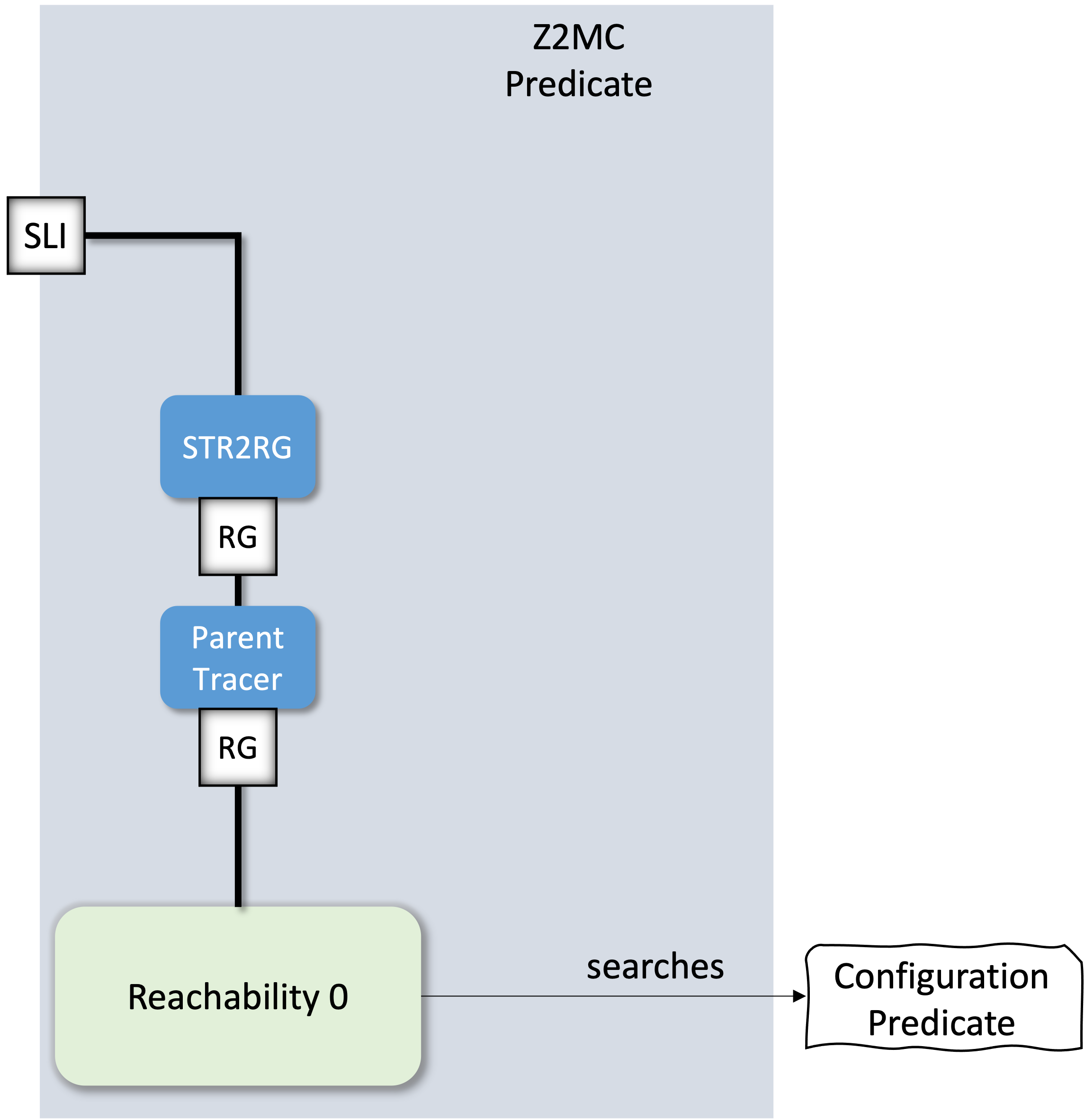
To simplify the manipulations these functions will be encapsulated in a new abstraction, which we name the SemanticTransitionRelation (STR).
-
Leslie Lamport. 1994. The temporal logic of actions. ACM Trans. Program. Lang. Syst. 16, 3 (May 1994), 872–923. https://doi.org/10.1145/177492.177726
-
Valentin Besnard, Matthias Brun, Frédéric Jouault, Ciprian Teodorov, and Philippe Dhaussy. 2018. Unified LTL Verification and Embedded Execution of UML Models. In Proceedings of the 21th ACM/IEEE International Conference on Model Driven Engineering Languages and Systems (MODELS '18). Association for Computing Machinery, New York, NY, USA, 112–122. https://doi.org/10.1145/3239372.3239395
-
Arthur Charguéraud, Adam Chlipala, Andres Erbsen, and Samuel Gruetter. 2023. Omnisemantics: Smooth Handling of Nondeterminism. ACM Trans. Program. Lang. Syst. 45, 1, Article 5 (March 2023), 43 pages. https://doi.org/10.1145/3579834
side question: Should we use RootedPiecewiseRelation instead of SemanticTransitionRelation?
class STR:
    def roots(self): pass
    def enabled(self, configuration): pass
    def execute(self, action, configuration): pass
To be able to reuse the algorithmic backend that we have already created, we need to somehow convert a STR to an RG abstraction. To achieve this, one approach is based on the Adapter design pattern. The adapter, named STR2RG, is another specialization of our RootedGraph abstraction that implements the RG API based on the STR API as follows:
class STR2RG:
    def __init__(self, anSTR):
        self.str = anSTR
    def roots(self):
        return self.str.roots()
    def neighbours(self, v):
        enabled_actions = self.str.enabled(v)
        targets = []
        for a in enabled_actions:
            targets += self.str.execute(a, v)
        return targets
With this setup we can already model interesting systems. Consider for instance the piecewise relation represented in the following graph:
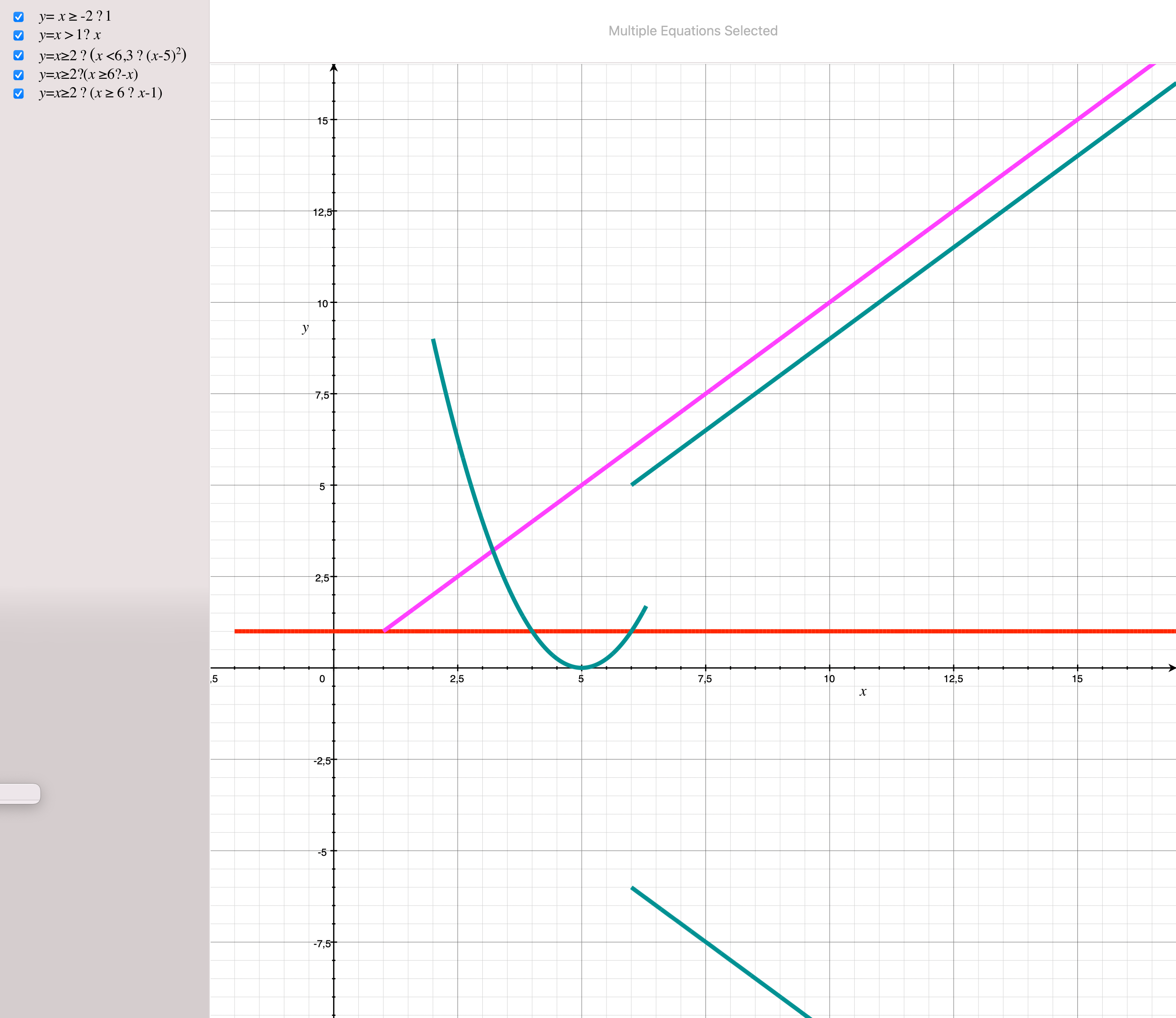
f(x) =
    - 1         if x ≥ -2
    - x         if x > 1
    - (x - 5)^2 if x ≥ 2 ∧ x < 6.3
    - -x        if x ≥ 2 ∧ x ≥ 6
    - x-1       if x ≥ 2 ∧ x ≥ 6
f(x) =
    - 1         if x ≥ -2
    - x         if x > 1
    - g(x) if x ≥ 2 ∧ g(x) =
        - (x - 5)^2 if x < 6.3
        - h(x) if x ≥ 6 ∧ h(x) =
            -x
            -x-1
This relation can be encoded with the STR-based intensional graph description as follows:
    class ExampleSTR:
        def roots(self):
            return [0]
        def enabled(self, configuration):
            x = configuration
            actions = []
            if (x >= -2):
                actions += [lambda x: [1]]
            if (x > 1):
                actions += [lambda x: [x]]
            if (x >= 2):
                actions += [lambda x:
                    r = []
                    if x < 6.3:
                        r.append((x-5)^2)
                    if x >= 6:
                        r.extend([-x, x-1])
                    r
            return actions
        def execute(self, action, configuration):
            return action(configuration)
Note that in the previous examples, we compute the new configuration (x') based on the previous value of x.
var x
init ≜ 0
next ≜ x' = 1      if x >= -2
    ∨  x' = x      if x >   1
    ∨   (   x' = (x-5)^2     if x < 6.3
        ∨   (x' = -x ∨ x' = x-1) if x >= 6) if x >= 2
spec ≜ init ∧ ☐next
//PiReDL syntax
def next (x) ≜
| x ≥ -2 ↦ 1
| x >  1 ↦ x
| x ≥  2 ↦
    | x < 6.3 ↦ (x-5)^2
    | x >= 6  ↦
        | -x
        | x - 1
Interesting side-note: Following the syntax 'idea' in the previous listing we can get to the TLA+ syntax rather naturally.
Existential quantification ∃ x ∈ S, condition ↦ S detect: λ x, condition
One simple yet interesting specification is a one-bit clock, which alternates forever between 0 and 1.
var clock
init ≜ clock = 0
     ∨ clock = 1
tick ≜ clock' = 1 if clock = 0
     ∨ clock' = 0 if clock = 1
spec ≜ init ∧ ☐tick
Flag Alice-Bob Another more interesting example will be the following specification trying to solve the binary mutual exclusion problem between Alice and Bob.
var a, b
init ≜ a = I ∧ b = I
alice ≜ a' = W if a = I
    ∨ a' = C if a = W ∧ b = I
    ∨ a' = I if a = C

bob ≜ b' = W if b = I
    ∨ b' = C if b = W ∧ a = I
    ∨ b' = I if b = C

spec = init ∧ ☐(alice ∨ bob)
Interesting side-note: As long as we are not concerned by specification refinement it is OK to disable stuttering: completely for safety verification and partially for liveness (stutter only on deadlock). With stuttering disabled the one-bit clock specification will disallow the behaviors where the clock never ticks.
0 → 0 → 0 → 0 → 0 → ...
1 → 1 → 1 → 1 → 1 → ...
Exercises
Exercise 1: Encode the previous specifications using the STR (like the ExampleSTR).
Exercise 2: Connect the STR2RG, ParentTracer and Reachability algorithm to implement a simple predicate verification setup.
Exercise 3: Use the verification setup to verify the mutual exclusion property []! (a = C ∧ b = C) on the following specification (Simple Alice-Bob):
var a, b
init ≜ a = I ∧ b = I
alice ≜ a' = C if a = I
    ∨ a' = I if a = C

bob ≜ b' = C if b = I
    ∨ b' = I if b = C

spec = init ∧ ☐(alice ∨ bob)
Exercise 4: Use the verification setup to verify that mutual exclusion property on the Flag Alice-Bob specification.
Exercise 5: Verify that Simple Alice-Bob and Flag Alice-Bob are deadlock-free. How can we encode the deadlock-freedom property?