
Foreword
This sequel is intended as a hands-on introduction to formal verification by model-checking (mostly explicit-state), even though a more sophisticated reader might see opportunities for symbolic or mixed explicit-symbolic verification.
After engaging with the content here a reader interested in using formal verification shall have the necessary background to understand deeply some of the existing model-checking tools: TLA+, SPIN, UPPAAL.
After engaging with the content here a reader working on language design might be willing to try designing (and implementing) the semantics of the language through the piecewise relation abstraction, which offers a bridge between behavioral language semantics (seen as specifications) and behavioral verification tools.
Games
- Teaching Model Checking via Games and Puzzles
- Model Checking Games and a Genome Sequence Search
- Principles of Model Checking: Regular Properties
Graph Traversal
Principles:
- Isolate the algorithms from the data structures they operate on.
- Explicitly state the hypotheses under which an algorithm works. And build up bridges toward satisfying those hypotheses.
In this chapter, we will introduce graphs and a graph traversal algorithm. We will keep it as simple as possible since the concepts here are well-known with rich literature.
 {: width="400" style="display:block; margin-left:auto; margin-right:auto"}
- Graph and Graph Representation
- [A] Graph Traversals -- [M] Explicit graph
- BFS
- Iterative
- Independent of the model
roots(); next() - OnEntry callback --> See another blog entry for a more generic version
Introducing the Rooted Graph
Graphs are among the most versatile and expressive structures in computer science. They naturally capture a wide range of relationships: from links between websites, to connections in a transportation network, to dependencies in a software project. However, while graphs are powerful, traversing them—systematically exploring their structure—is far from trivial.
One key insight in building robust traversal algorithms is recognizing that how a graph is represented should not affect the traversal logic. In other words, our algorithms should not be entangled with specific data structures. This separation of concerns is not just a matter of good software engineering—it is essential if we want our tools to scale across domains, adapt to new applications, and support multiple input formats.
Yet, there's a more fundamental problem. In many real-world cases, we're not simply interested in an arbitrary traversal of a graph. We want to explore a particular part of it, starting from certain points of interest and systematically branching out. This requirement naturally leads us to a structure that we call a rooted graph.
A rooted graph is not just a graph, it is a graph together with a distinguished set (or multiset) of roots. These roots represent the starting points of traversal. They might correspond to known initial states in a system, entry nodes in a program's control flow, or nodes we suspect are critical in a network. By explicitly incorporating the notion of roots, we make a commitment: we are not trying to understand the entire graph blindly, but to explore what can be reached and discovered from known anchors.
This view immediately raises the question: how do we best represent such a rooted graph? There is no universally optimal way to store a graph. Sparse graphs benefit from adjacency lists, dense ones may do better with matrices, and large-scale graphs might be stored in files or streamed from a database. The rooted graph abstraction allows us to factor out the representation details and focus on what matters: the reachable structure from a set of entry points.
In doing so, we create a flexible interface for algorithms. An algorithm that operates on rooted graphs needs only to know two things: how to obtain the roots, and how to get the neighbors of a given vertex. Everything else (the storage, the indexing, even the vertex types) becomes an implementation detail. This minimal contract is sufficient to power sophisticated traversals, verifications, and ultimately the core mechanisms behind model-checking.
In this chapter, we will progressively build this abstraction, beginning with simple, explicit graphs, and moving toward more expressive and efficient representations. Along the way, we will isolate our traversal algorithms from specific data structures, creating a flexible foundation for the rest of the book.
Expanding the Rooted Graph Concept: Extrinsic vs. Intrinsic Graphs
The notion of a rooted graph brings us a step closer to modular, general-purpose traversal algorithms. But it also opens the door to a deeper realization: not all graphs are known in advance.
Some graphs are extrinsic: they are explicitly represented, stored in memory or on disk, with their vertices and edges fully known before any traversal begins. These are the typical graphs that one might find in textbooks or programming assignments: adjacency matrices, edge lists, and hash maps. In such cases, all of the data is available up front, and the graph is simply a static data structure to be navigated.
However, many graphs we care about in model-checking are intrinsic. They are not fully constructed before use, nor are they even necessarily finite. Instead, these graphs are defined procedurally. Their structure is revealed step-by-step as we traverse them, with each expansion generating new nodes and edges on the fly. Think of the state space of a program: it is often far too large (or even infinite) to be built explicitly, yet we can compute the successors from any given state.
To make this concept more concrete, consider the example of walking a social network graph using internet requests. Suppose you start from a single user and wish to explore their connections: friends, friends of friends, and so on. Each node in the graph represents a user profile, and edges represent "friend" relationships. But the graph is not known in advance. Instead, each node's neighbors are discovered by querying a server for that user's friends. This is a classic intrinsic graph: its vertices and edges are fetched lazily, on-demand, during traversal. If the traversal stops early (e.g., after finding a particular person or after a certain depth), large parts of the graph remain unexplored and unmaterialized.
This is where the rooted graph abstraction shines. By requiring only two capabilities from a graph, (1) the ability to provide a set of roots, and (2) the ability to compute the neighbors of a vertex, we enable traversals that work seamlessly over both extrinsic and intrinsic graphs.
This abstraction lets us unify a broad class of graphs under a common interface. Whether the graph is a static list of nodes and edges read from a file, or a dynamic exploration of system states driven by simulation or symbolic execution, the traversal algorithm sees only the operations it needs.
In later sections, we will see how this perspective allows us to apply the same core traversal logic to a wide range of applications: from solving games like the Tower of Hanoi, to verifying reachability properties in software models. The rooted graph interface becomes the contract between the traversal algorithm and the underlying system—regardless of whether that system is fully known or just gradually revealed.
This perspective, of graphs not just as data, but as behaviors, is foundational to the rest of the book.
A Rooted Graph and an Explicit Graph Data Structure
A graph is defined as a tuple G=(V, E) where V is an arbitrary set of vertices, and E is a binary relation between the elements in V.
For technical reasons, that will become apparent later, we will allow both self-loops and duplicate edges.
For our purposes, we enrich the previous graph definition with R ⊆ V the multiset of roots of the graph. The roots of a graph are the vertices that provide access to the connected components of the graph. Sometimes R can be just a set, however, the more relaxed multiset concept allows for simpler, less constrained implementations (a list of nodes for instance).
Thus a rooted graph RG is defined as RG=(V, E, R).
Dictionary-based Rooted Graph
To make it simple, we will represent the rooted graph structure by encoding the graph as an adjacency list using a dictionary. The keys of the dictionary will be the vertices of the graph. To each vertex we will associate a list of nodes, which are directly reachable from the vertex.
graph = {
  1: [2, 3],
  2: [3, 4]
}
To obtain the rooted graph structure we complement the dictionary with another list of vertices, the roots.
roots = [1, 2].
The rooted graph structure is then obtained by encapsulating these to fields in an object. Let's first define a DictionaryRootedGraph class, which allows building the objects that we need.
class DictionaryRootedGraph:
  def __init__(self, graph, roots):
    self.graph = graph
    self.roots = roots
With this, we already have a small domain-specific language (embedded in Python), which allows us to build rooted graphs. Let's see an example
graph1 = DictionaryRootedGraph(
    {
        1: [2, 3],
        2: [3, 4]
    },
    [1, 3]
)
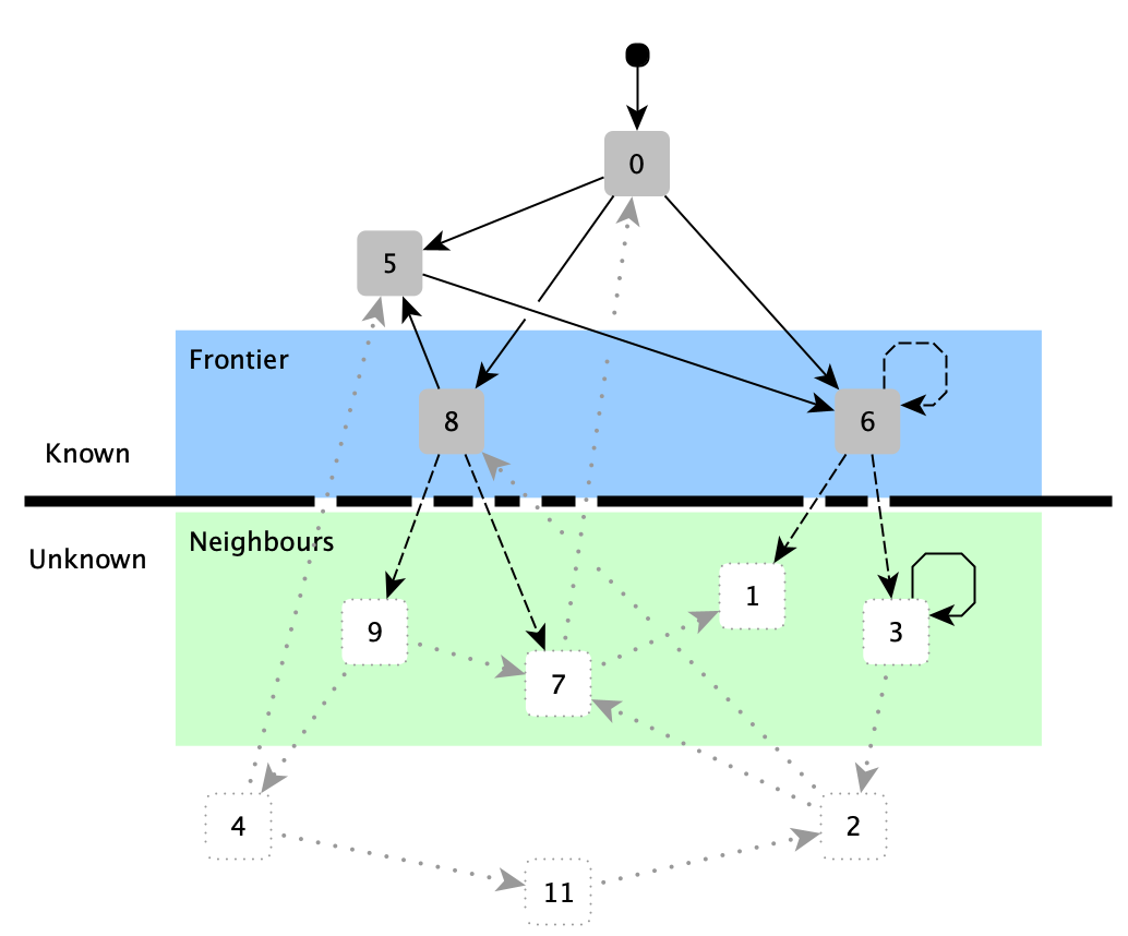
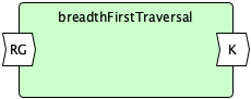
Breadth-First Traversal
 {: width="400" style="display:block; margin-left:auto; margin-right:auto"}
traversal K {}      = K
traversal K {x} ∪ F = traversal K F                            if x ∈ K
traversal K {x} ∪ F = traversal ({x} ∪ K) ((neighbors x) ∪ F)  if x ∉ K

dfs K []        = K
dfs K (x::L)    = dfs K L                            if x ∈ K
dfs K (x::L)    = dfs ({x} ∪ K) ((neighbors x) ++ L) if x ∉ K

bfs K []        = K
bfs K (x::L)    = dfs K L                            if x ∈ K
bfs K (x::L)    = dfs ({x} ∪ K) (L ++ (neighbors x)) if x ∉ K
 {: width="200" style="display:block; margin-left:auto; margin-right:auto"}
breadthFirstTraversal(rootedGraph):
    I = True
    K = ∅
    F = []
    WHILE F ≠ ∅ ∨ I DO
        N = IF I THEN rootedGraph.roots ELSE rootedGraph.graph[F.dequeue()]
        I = False
        FORALL n ∈ N
            IF n ∉ K THEN
                K = K ∪ {n}
                F = F ∪ {n}
    RETURN K
NOTE: For implementing a set in Python use the set data structure.
NOTE: For implementing the FIFO queue in Python use the deque (Double-Ended Queue) data structure data structure. The deque is a list-like sequence optimized for data access near its endpoints.
Implement this algorithm in Python, and test it. Don't forget to use the debugger to understand what is happening. Amongst your tests think of edge cases for instance:
breadthFirstTraversal(DictionaryRootedGraph())breadthFirstTraversal(DictionaryRootedGraph({}, nil))breadthFirstTraversal(DictionaryRootedGraph(nil, []))breadthFirstTraversal(DictionaryRootedGraph({1: nil}, []))
Fix the algorithm to pass all tests.
Abstracting Over the Graph
Why is the algorithm polluted with the implementation details of the DictionaryRootedGraph?
The key idea here is to look at the algorithm implementation and try to abstract over the queries on the DictionaryRootedGraph data structure by introducing methods, which will hide the data structure-specific details. We need to analyze the algorithm to understand what queries it performs on our data structure. In our case, the answer is rather simple since our breadthFirstTraversal uses the rootedGraph only at line 6, where performs two queries:
- If we are at the beginning (during the initialization phase), we need the roots of the graph - our entries in the graph.
- In the subsequent steps, for any vertex
vobtained from the frontier (F.dequeue()) we need to obtain its neighbors (the vertices that we get by following the edges starting atv).
Let's add these two methods to the DictionaryRootedGraph class, and then update the breadthFirstTraversal to use these methods, instead of directly using instance variable accesses.
class DictionaryRootedGraph:
    def __init__(self, graph, roots):
        self._graph = graph
        self._roots = roots

    def roots(self):
        return self._roots

    def neighbors(self, vertex):
        return self._graph[vertex]
Different Data Structures
Let's say now that we don't like this rooted graph implementation because I have better data-structure implementations:
- for dense graphs (graphs with many edges) a Matrix (a bitmap) representation will be more compact.
- for large graphs with few edges, a sparse matrix encoding of the graph is more compact.
- storing the edges explicitly in a list is easy to parse.
To allow our algorithm to work with different encodings of the graph
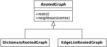
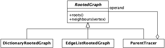
Based on this analysis, we can introduce the abstract concept of RootedGraph that will encapsulate (group together) these two functions.
class RootedGraph:
    def roots(self): pass
    def neighbors(self, vertex): pass
NOTE: By inheriting from ABC and adding the @abstractmethod annotation we can ensure that the RootedGraph abstract class cannot be instantiated directly.
Python uses the duck-typing principle: "If it walks like a duck and it quacks like a duck, then it must be a duck".
Following this principle, in our case, that means that any object that implements the roots(self) and next(self, vertex) methods are considered implicitly as instances of the RootedGraph abstract class. Furthermore, we do not need to define the RootedGraph abstract class at all. Nevertheless doing so greatly improves the readability of the code, as the abstract class clearly defines the public API of any RootedGraph instance. To be even more explicit we can explicitly define the DictionaryRootedGraph class to be an instance of the RootedGraph abstract class.
class DictionaryRootedGraph(RootedGraph):
The EdgeListRootedGraph is a different data structure that can represent the graph with a simple list of edges. The edges in the list are encoded as a Python tuple (source, destination), where the source object represents the source vertex of the edge and the destination object represents the target vertex of the edge.
Besides the edge list, our `RootedGraph`` needs the roots of the graph, we will represent them as a list as earlier.
Create the EdgeListRootedGraph
Here is a simple graph
graph = EdgeListRootedGraph(
    [
        (1, 2),
        (1, 3),
        (2, 3),
        (2, 4)
    ],
    [1,3]
)
What do we need to do so that we can use our BFS algorithm with this new data structure?
What are the differences between the DictionaryRootedGraph and the EdgeListRootedGraph?
The EdgeListRootedGraph instances are easier to create from a file containing the roots and the edge list.
1 3 #roots
1 2
1 3
2 3
2 4
Write a reader factory that creates an EdgeListRootedGraph from such a file.
 {: width="400" style="display:block; margin-left:auto; margin-right:auto"}
More Generic Vertex Types
Up until now, we have used only integer objects to represent the graph vertices. But in the long run, we will want to handle generic objects.
Try creating a graph of Persons(first_name, family_name) identified by their name. The relations in the graph represent that a Person knows another Person.
Run the previous reachability algorithm on this graph. If we have a relation Person(a, b) -> Person(a, b) what is the result of the reachability query? Why do we have Person(a, b) twice in the result? How can we fix that?
Object Identity versus object Equality, and the set implementation in Python.
To solve this problem we need to enrich our objects with a domain-specific notion of equality. What makes two Person instances equal?
class Person:
    ...
    def __eq__(self, other):
        ...
    def __hash__(self):
        ...
Breadth-First Search
 {: width="200" style="display:block; margin-left:auto; margin-right:auto"}
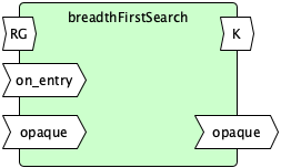
breadthFirstSearch(graph, on_entry, opaque):
    I = True
    K = ∅
    F = []
    WHILE F ≠ ∅ ∨ I DO
        N = IF I THEN graph.roots() ELSE graph.neighbours(F.dequeue())
        I = False
        FORALL n ∈ N
            IF n ∉ K THEN
                terminate = on_entry(n, opaque)
                IF terminate THEN
                    RETURN (opaque, K)
                K = K ∪ {n}
                F = F ∪ {n}
    RETURN (opaque, K)
Intensional Graphs: Hanoi Example
 {: width="400" style="display:block; margin-left:auto; margin-right:auto"}
Up until now, we have used only extensional graph representations. But there is no fundamental limit precluding us from using also intensional graph representations. These are graphs that are defined by giving a procedure that can be followed to obtain the graph dynamically on request. At this point, we will start to see the power of our query-based graph manipulations. Here instead of enumerating all the vertices and edges of the graph, we will provide smart implementation of the roots and neighbors methods to generate special graphs programmatically that will then be analyzed by our algorithms.
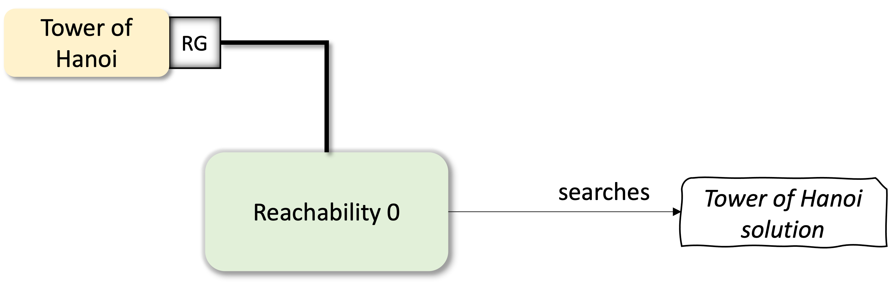
To make this section a bit concrete we will create a NBits game. The aim is to encode the game state as graph vertices and the game actions, that link two game states, as edges. After encoding the game rules we will look for the solution by simply calling our breadth-first search algorithm.
class NBits:
    def __init__(self, n, ini: list):
        self.n = n
        self.ini = ini
        self.accepting = accepting

    def roots(self):
        return self.ini

    def neighbors(self, configuration: int):
        targets = []
        for i in range(self.n):
            if ((configuration >> i) & 1) > 0:
                target = configuration & ~(1 << i)
            else:
                target = configuration | (1 << i)
            targets.append(target)
        return targets
Now we have these steps to follow:
- Define what is a configuration
def __eq__(self, other):def __hash__(self):
- Define the rooted graph API
- what is the list of roots?
- write an algorithm that generates the neighbors of a given configuration
- Define the query
if __name__ == '__main__':
    nbits = NBits(10, [0])
    (target, k) = bfsSearch(nbits, lambda x: x == 5)
Exercise:
- Implement Tower of Hanoi Game
Practical situation: Going beyond simple search. Giddy, Jonathan P., and Reihaneh Safavi-Naini. "Automated cryptanalysis of transposition ciphers." The Computer Journal 37.5 (1994): 429-436.
This is great, but, how did we get to this solution?
Building the Trace
 {: width="400" style="display:block; margin-left:auto; margin-right:auto"}
 {: width="400" style="display:block; margin-left:auto; margin-right:auto"}
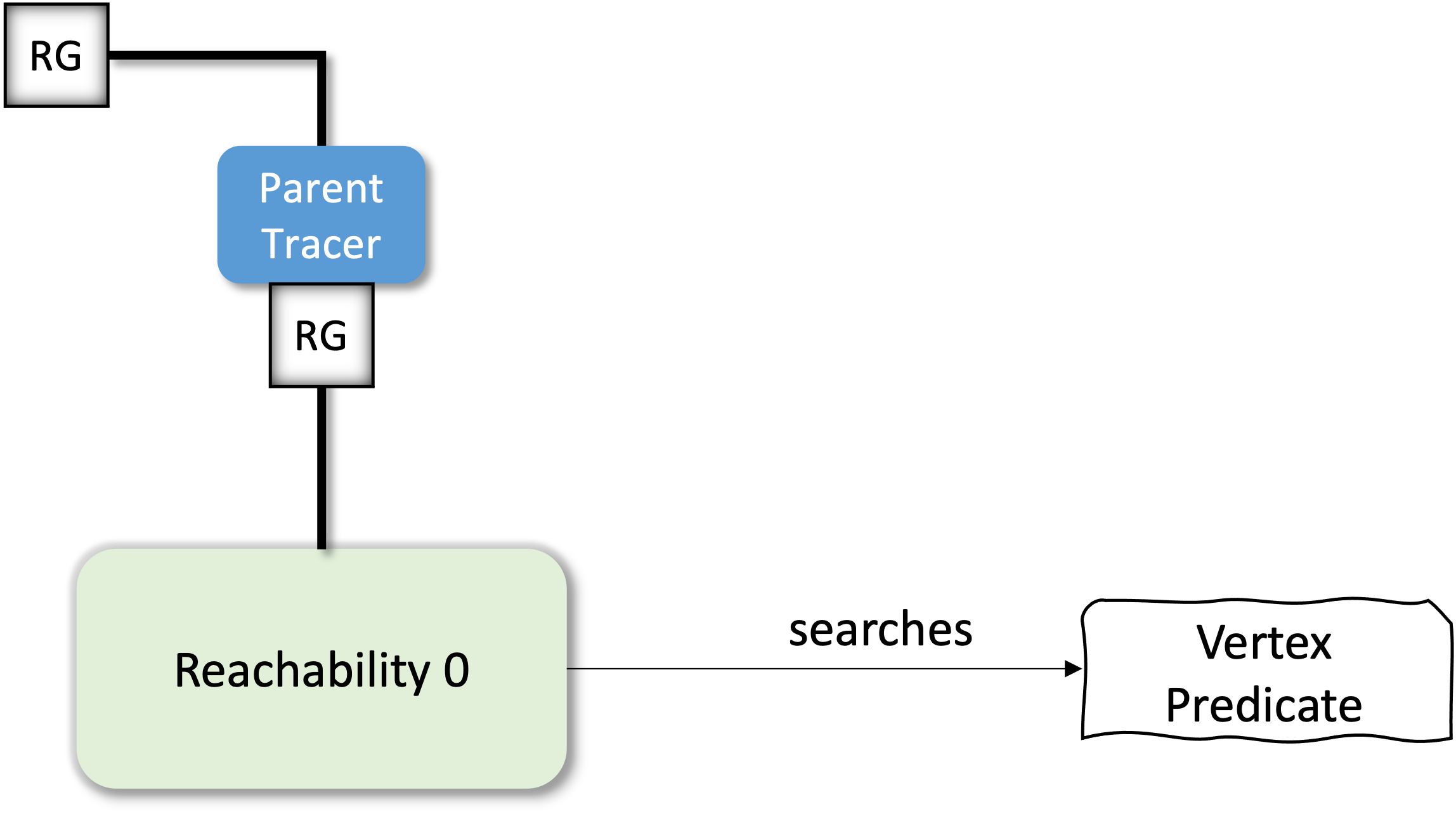
class ParentTracer(RootedGraph):

    def __init__(self, operand, parents=None):
        self.operand = operand
        self.parents = {} if parents is None else parents

    def roots(self):
        neighbours = self.operand.roots()
        for n in neighbours:
            self.parents[n] = []
        return neighbours

    def neighbors(self, vertex):
        neighbours = self.operand.neighbors(vertex)
        for n in neighbours:
            if self.parents.get(n) is None:
                self.parents[n] = [vertex]
        return neighbours
Piecewise Relations
 {: width="400" style="display:block; margin-left:auto; margin-right:auto"}
The intensional graph description used in the previous section allowed us to economically encode a whole family of domain-specific graphs (ie. The graphs representing the valid moves allowed by the Tower of Hanoi puzzle). There are two downsides with this approach that we want to emphasize in this section:
- The rooted graph abstraction that we have used abstracts over the graph edges, which leads to an imprecise encoding of graphs with edge annotations. Different workarounds are still possible:
- define another function
edge_data(source, target)->maybe(annotation)that retrieves the annotation from any pair of related vertices. But this approach precludes multiple edges between two vertices (a,b,x) (a,b,y). - encode the graph of interest differently, ie push the edge annotation to the target vertex. But this can result in an exponential blowup in the resulting graph.
- define another function
- The implementation of the
neighboursfunction in the Tower of Hanoi example has multiple responsibilities:- detect if a disk move is possible
- create the target configuration/vertex. Typically it is cheaper to create the target configuration by
- copying the source configuration
- changing it according to the move considered
To address these limitations we will first decompose the neighbours function in two parts:
- an
enabled: C → set Afunction that enables to detect the transitions (edges) allowed in the current configuration. - an
execute: A → C → set Cfunction that interprets an enabled transition to obtain the target configuration.
This decomposition leads us to an abstraction closely resemblinng piecewise functions. In mathematics piecewise functions allow the definition of functions by parts, where each part is a function enabled under a specific condition. To ensure that the resulting piecewise definition is still a function the set of conditions need to be mutually exclusive. We will not enforce this exclusivity constraint which leads to the more generic piecewise relation abstraction. Furthermore, we also relax the functional constraint on the parts too. Thus we get to a very general definition of a piecewise relation, where each part itself is a relation, potentially defined piecewise itself.
Important: Please note that both enabled and execute are functions with sets as codomains.
Note that we can also define the predicate enabled: A → C → bool, which returns true if an action A is enabled in the configuration C.
To simplify the manipulations these functions will be encapsulated in a new abstraction, which we name the SemanticTransitionRelation (STR).
-
Leslie Lamport. 1994. The temporal logic of actions. ACM Trans. Program. Lang. Syst. 16, 3 (May 1994), 872–923. https://doi.org/10.1145/177492.177726
-
Valentin Besnard, Matthias Brun, Frédéric Jouault, Ciprian Teodorov, and Philippe Dhaussy. 2018. Unified LTL Verification and Embedded Execution of UML Models. In Proceedings of the 21th ACM/IEEE International Conference on Model Driven Engineering Languages and Systems (MODELS '18). Association for Computing Machinery, New York, NY, USA, 112–122. https://doi.org/10.1145/3239372.3239395
-
Arthur Charguéraud, Adam Chlipala, Andres Erbsen, and Samuel Gruetter. 2023. Omnisemantics: Smooth Handling of Nondeterminism. ACM Trans. Program. Lang. Syst. 45, 1, Article 5 (March 2023), 43 pages. https://doi.org/10.1145/3579834
side question: Should we use RootedPiecewiseRelation instead of SemanticTransitionRelation?
class STR:
    def roots(self): pass
    def enabled(self, configuration): pass
    def execute(self, action, configuration): pass
To be able to reuse the algorithmic backend that we have already created, we need to somehow convert a STR to an RG abstraction. To achieve this, one approach is based on the Adapter design pattern. The adapter, named STR2RG, is another specialization of our RootedGraph abstraction that implements the RG API based on the STR API as follows:
class STR2RG:
    def __init__(self, anSTR):
        self.str = anSTR
    def roots(self):
        return self.str.roots()
    def neighbours(self, v):
        enabled_actions = self.str.enabled(v)
        targets = []
        for a in enabled_actions:
            targets += self.str.execute(a, v)
        return targets
With this setup we can already model interesting systems. Consider for instance the piecewise relation represented in the following graph:
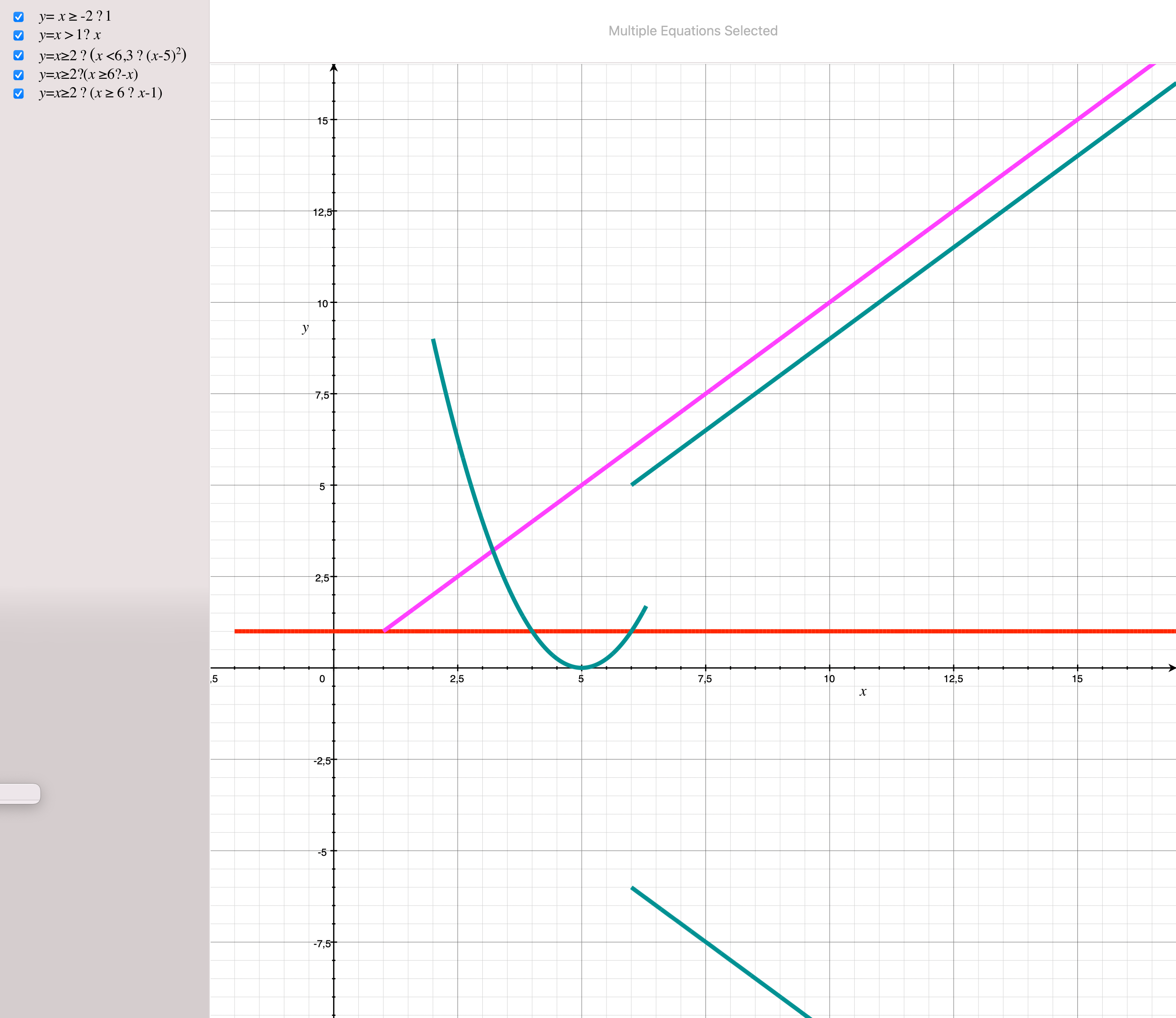
f(x) =
    - 1         if x ≥ -2
    - x         if x > 1
    - (x - 5)^2 if x ≥ 2 ∧ x < 6.3
    - -x        if x ≥ 2 ∧ x ≥ 6
    - x-1       if x ≥ 2 ∧ x ≥ 6
f(x) =
    - 1         if x ≥ -2
    - x         if x > 1
    - g(x) if x ≥ 2 ∧ g(x) =
        - (x - 5)^2 if x < 6.3
        - h(x) if x ≥ 6 ∧ h(x) =
            -x
            -x-1
This relation can be encoded with the STR-based intensional graph description as follows:
    class ExampleSTR:
        def roots(self):
            return [0]
        def enabled(self, configuration):
            x = configuration
            actions = []
            if (x >= -2):
                actions += [lambda x: [1]]
            if (x > 1):
                actions += [lambda x: [x]]
            if (x >= 2):
                actions += [lambda x:
                    r = []
                    if x < 6.3:
                        r.append((x-5)^2)
                    if x >= 6:
                        r.extend([-x, x-1])
                    r
            return actions
        def execute(self, action, configuration):
            return action(configuration)
Note that in the previous examples, we compute the new configuration (x') based on the previous value of x.
var x
init ≜ 0
next ≜ x' = 1      if x >= -2
    ∨  x' = x      if x >   1
    ∨   (   x' = (x-5)^2     if x < 6.3
        ∨   (x' = -x ∨ x' = x-1) if x >= 6) if x >= 2
spec ≜ init ∧ ☐next
//PiReDL syntax
def next (x) ≜
| x ≥ -2 ↦ 1
| x >  1 ↦ x
| x ≥  2 ↦
    | x < 6.3 ↦ (x-5)^2
    | x >= 6  ↦
        | -x
        | x - 1
Interesting side-note: Following the syntax 'idea' in the previous listing we can get to the TLA+ syntax rather naturally.
Existential quantification ∃ x ∈ S, condition ↦ S detect: λ x, condition
One simple yet interesting specification is a one-bit clock, which alternates forever between 0 and 1.
var clock
init ≜ clock = 0
     ∨ clock = 1
tick ≜ clock' = 1 if clock = 0
     ∨ clock' = 0 if clock = 1
spec ≜ init ∧ ☐tick
Flag Alice-Bob Another more interesting example will be the following specification trying to solve the binary mutual exclusion problem between Alice and Bob.
var a, b
init ≜ a = I ∧ b = I
alice ≜ a' = W if a = I
    ∨ a' = C if a = W ∧ b = I
    ∨ a' = I if a = C

bob ≜ b' = W if b = I
    ∨ b' = C if b = W ∧ a = I
    ∨ b' = I if b = C

spec = init ∧ ☐(alice ∨ bob)
Interesting side-note: As long as we are not concerned by specification refinement it is OK to disable stuttering: completely for safety verification and partially for liveness (stutter only on deadlock). With stuttering disabled the one-bit clock specification will disallow the behaviors where the clock never ticks.
0 → 0 → 0 → 0 → 0 → ...
1 → 1 → 1 → 1 → 1 → ...
Exercises
Exercise 1: Encode the previous specifications using the STR (like the ExampleSTR).
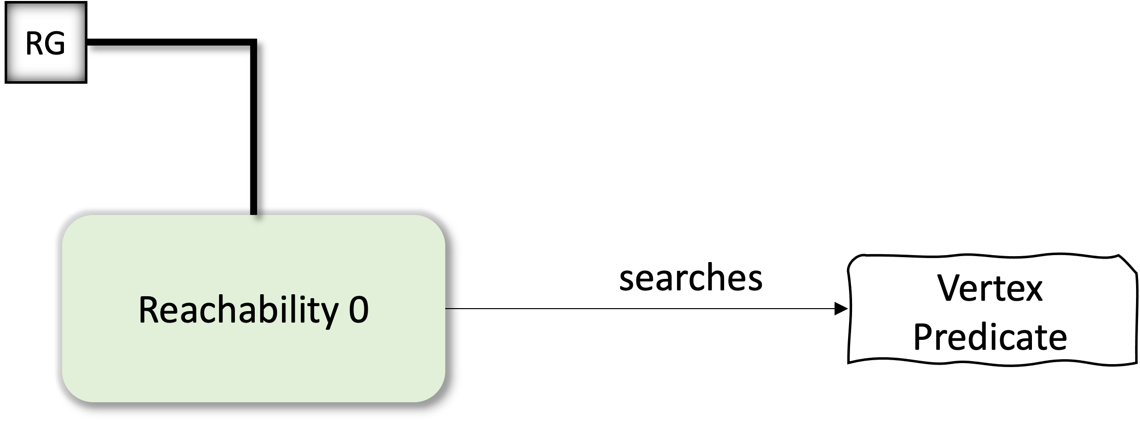
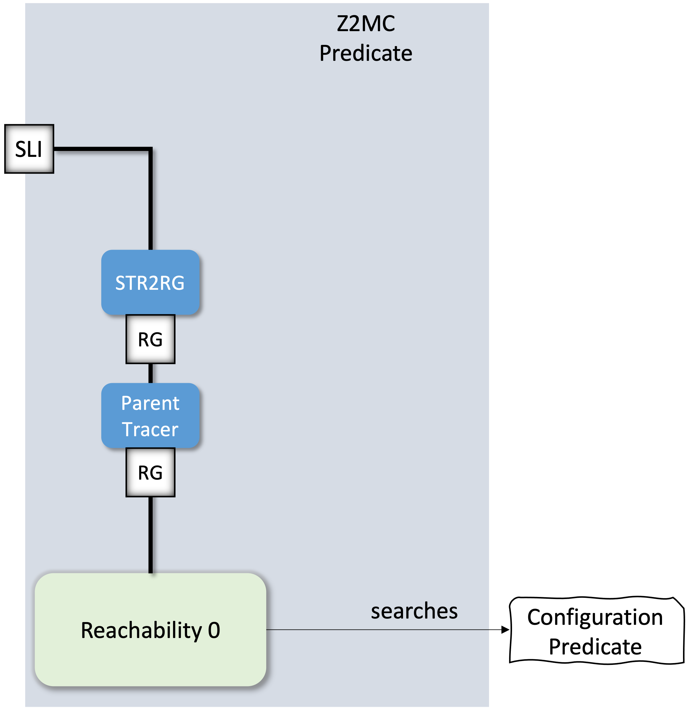
Exercise 2: Connect the STR2RG, ParentTracer and Reachability algorithm to implement a simple predicate verification setup.
Exercise 3: Use the verification setup to verify the mutual exclusion property []! (a = C ∧ b = C) on the following specification (Simple Alice-Bob):
var a, b
init ≜ a = I ∧ b = I
alice ≜ a' = C if a = I
    ∨ a' = I if a = C

bob ≜ b' = C if b = I
    ∨ b' = I if b = C

spec = init ∧ ☐(alice ∨ bob)
Exercise 4: Use the verification setup to verify that mutual exclusion property on the Flag Alice-Bob specification.
Exercise 5: Verify that Simple Alice-Bob and Flag Alice-Bob are deadlock-free. How can we encode the deadlock-freedom property?
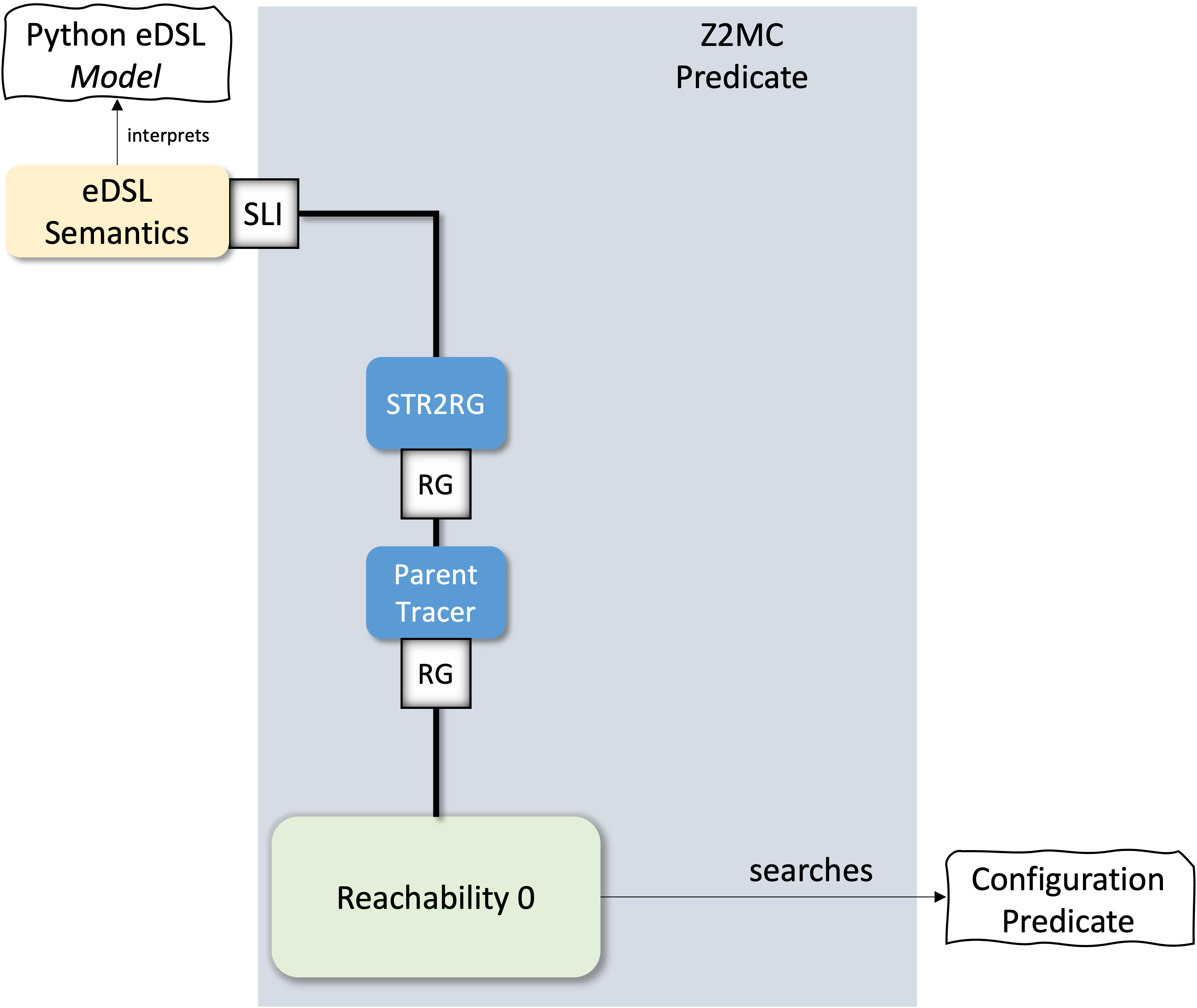
A Simple Python eDSL for Piecewise Relations
 {: width="400" style="display:block; margin-left:auto; margin-right:auto"}
Implementing the STR directly works, but looking at our last specifications using the made-up language we see that there is a certain syntactical pollution. To address this issue in this chapter we will create a simple embedded Domain-Specific Language (eDSL) in Python.
Note: Creating an external DSL for our specification language is outside the scope of this work. The interested reader is nevertheless encouraged to try. Such a reader is encouraged to study the TLA+ syntax to find other (rather inspired) operators, which can further simplify the syntax. Readers keen on the graphical syntax could study UML statecharts in conjunction with the AnimUML specification and verification environment to get another more graphical perspective.
Our eDSL will be named Soup, because it will encode the specifications as a soup of pieces necessary to encode the piecewise relations.
The first ingredient, which will encode the valuation of the variables used in a specification is identical to the Configuration concept that we have used for generalizing the Vertex types in the graph abstraction.
For the one-bit clock example we will have:
class OneBitClockConfig:
    def __init__(self, value):
        self.clock = value

    def __hash__(self):
        return hash(self.clock)

    def __eq__(self, other):
        if not isinstance(other, OneBitClockConfig):
            return False
        return self.clock == other.clock

    def __repr__(self):
        return f'clock={self.clock}'
The initialization part of the specification can be decomposed around the disjunctions. Each term in the disjunction will become a unique configuration. Moreover, each such term is required to initialize all the variables. Thus the initialization of the one-bit clock will be defined as follows:
init = [OneBitClockConfig(0), OneBitClockConfig(1)]
Each piece of the relation will be encoded as two lambdas encapsulated in a LambdaPiece object, defined as follows:
class LambdaPiece:
    def __init__(self, name='', guard, generator):
        self.name = name
        self.guard = guard
        self.generator = generator

    def __eq__(self, other):
        if not isinstance(other, LambdaPiece):
            return False
        return self.name == other.name and self.guard == other.guard and self.generator == other.generator
For the one-bit clock specification, we get:
toOne  = LambdaPiece('toOne',  lambda c: OneBitClockConfig(1), lambda c: c.clock == 0)
toZero = LambdaPiece('toZero', lambda c: OneBitClockConfig(0), lambda c: c.clock == 1 )
The specification is captured in a Soup instance, defined as follows:
class Soup:
    def __init__(self, initial=[], pieces=[]):
        self.initial = initial
        self.pieces = pieces

    def add(self, name, guard, generator):
        self.extend(LambdaPiece(name, guard, generator))

    def extend(self, beh):
        if isinstance(beh, LambdaPiece):
            self.pieces.append(beh)
        else:
            self.pieces.extend(beh)
For the one-bit clock specification, the soup is:
one_bit_clock_spec = Soup(init, [toOne, toZero])
To interpret the soup as a piecewise relation, the next step is to implement the semantics as follows:
class RootedPiecewiseRelationSemantics(SemanticTransitionRelation):
    def __init__(self, soup):
        self.soup = soup

    def roots(self):
        return self.soup.initial

    def enabled(self, configuration):
        return list(filter(lambda ga: ga.guard(configuration), self.soup.pieces))

    def execute(self, action, configuration):
        target = copy.deepcopy(configuration)
        the_output = action.generator(target)
        return the_output
Note that in the implementation of the execute function we perform a deepcopy. Is this necessary? Knowing that the generator lambda produces a new configuration each time. Explain and give an example where this is necessary.
By the way, the one-bit specification can be even shorter:
one_bit_clock_spec = Soup(
    [0, 1],
    [
        LambdaPiece('toOne',  lambda c: 1, lambda c: c == 0),
        LambdaPiece('toZero', lambda c: 0, lambda c: c == 1)
    ]
)
Why does it work? Can you explain why we do not strictly need a Configuration object in this case?
It can be rather similar to the spec in the previous chapter if written as follows:
init = [0, 1]
tick = [
        LambdaPiece(lambda c: 1, lambda c: c == 0),
        LambdaPiece(lambda c: 0, lambda c: c == 1)]
spec = Soup(init, tick)
Exercises
Exercise 1: Encode the specifications from the previous chapter using the Soup language. Exercise 2: Create a predicate verification tool for the Soup language.
Exercise 3: Verify the mutual exclusion property on the Soup-based Simple Alice-Bob specification.
Exercise 4: Verify the mutual exclusion property on the Soup-based Flag Alice-Bob specification.
Exercise 5: Verify that Simple Alice-Bob and Flag Alice-Bob are deadlock-free.
Make sure that the results match the ones obtained in the previous chapter. If they don't match find and fix the bugs.
Exercise 6: Encode the Hanoi problem using the Soup language and use the Soup predicate verifier to find the solution.
Exercise 7: TODO: German traffic light and history management.
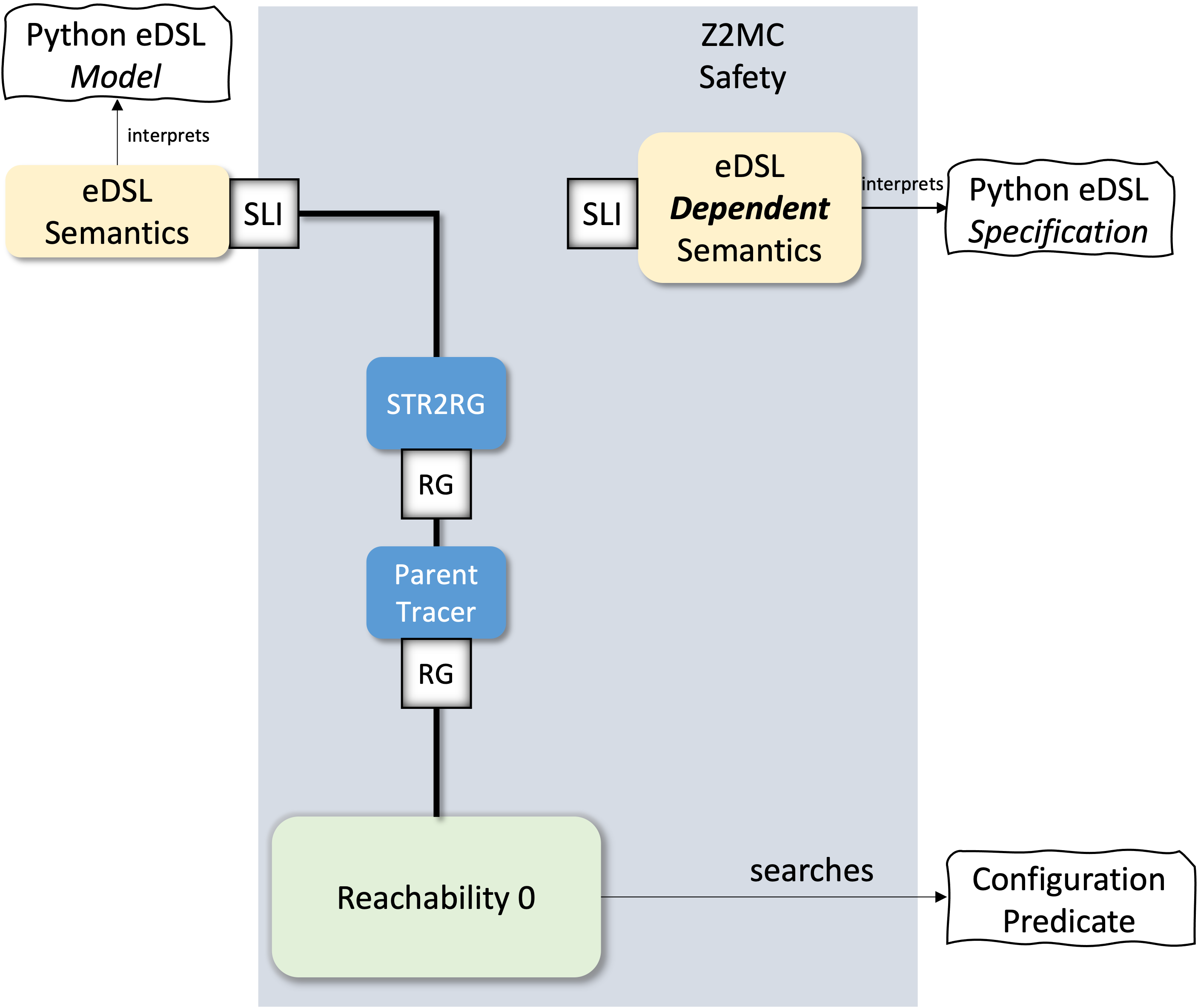
More Expressive Properties Through Dependent Semantics
 {: width="400" style="display:block; margin-left:auto; margin-right:auto"}
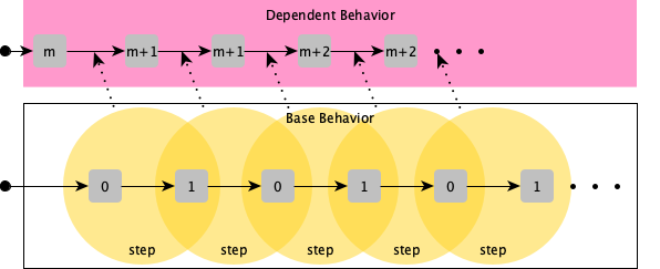
Until now our verification tasks were limited to predicate verification. To go further we need to extend the expressivity of the "property" language, which was restricted to simple state predicates. To achieve this we will first extend our semantical framework to allow the creation of dependencies between different semantics. The discussion in this chapter is based on the Soup language, which is extended to allow the design of dependent specifications.
One case where dependent semantics can came in handy is specifying the behaviour of a minute clock based on the ticks of the one-bit clock. The minute variable should be incremented on the rising edge of the one-bit clock.
var minutes
init ≜ minutes ∈ {1..60}             -- note the non-deterministic assignement
tick ≜ minutes' = (minutes + 1) % 60 + 1 if clock = 0 ∧ clock' = 1
spec ≜ init ∧ ☐(tick ∨ minutes' = minutes)
 {: style="display:block; margin-left:auto; margin-right:auto"}
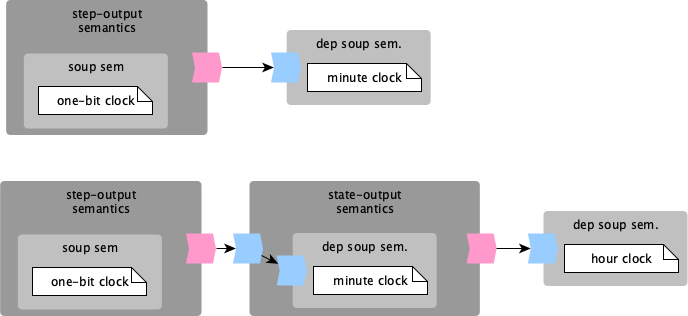
Another example is the hour clock based on the minute clock.
var hour
init ≜ hour ∈ {1..12}             -- note the non-deterministic assignement
tick ≜ hour' = (hour + 1) % 12 + 1 if minutes = 60
spec ≜ init ∧ ☐(tick ∨ hour' = hour)
If we are looking at these previous specification they seem incomplete. The minute clock specification defines its behaviour relatively to another behavior, from which it can extract a notion of clock. The name clock is used in the minute-clock but its behaviour is never defined.
 {: style="display:block; margin-left:auto; margin-right:auto"}
We define a dependent semantics as a semantics that requires some additional input (of type I), besides the current configuration (of type C), to:
- decide what is the set of enabled actions. If The
actionsfunction signature becomesactions: I → C → set A. - compute the target configuration set, during the execution of an action. The
executesignature becomesexecute: A → I → C → set C.
Now that we have an input-dependent semantics, we can define an output producing semantics to improve the symmetry of our design. Such a semantics should produce an output during the execution of a step, in such a way that is possible to connect it to the an input-dependent semantics. To achieve this, we extend the signature of the execute function: execute: A → I → C → set (O × C). During the execution of an action an output O is produced, besides the new configuration.
With these two ideas our semantically framework evolves, to something very similar to Mealy abstract machines. The execution step is dependent on the current configuration, and the input. Action execution effectivelly computes the next comfiguration and the output. Thus a step in the semantics state-space becomes:
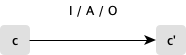 {: style="display:block; margin-left:auto; margin-right:auto"}
class RootedPiecewiseRelationDependentSemantics:

    def __init__(self, soup):
        self.soup = soup

    def roots(self):
        return self.soup.initial

    def enabled(self, input, configuration):
        return list(filter(lambda ga: ga.guard(input, configuration), self.soup.pieces))

    def execute(self, action, input, configuration):
        target = copy.deepcopy(configuration)
        the_output = action.generator(input, target)
        return the_output
class ToStepOutputSemantics:

    def __init__(self, subject):
        self.subject = subject

    def roots(self):
        return self.subject.initial

    def enabled(self, configuration):
        return self.subject.enabled

    def execute(self, action, configuration):
        the_targets = self.subject.execute(action, configuration)

        return list(map(lambda t: ((configuration, action, t), t), the_targets))
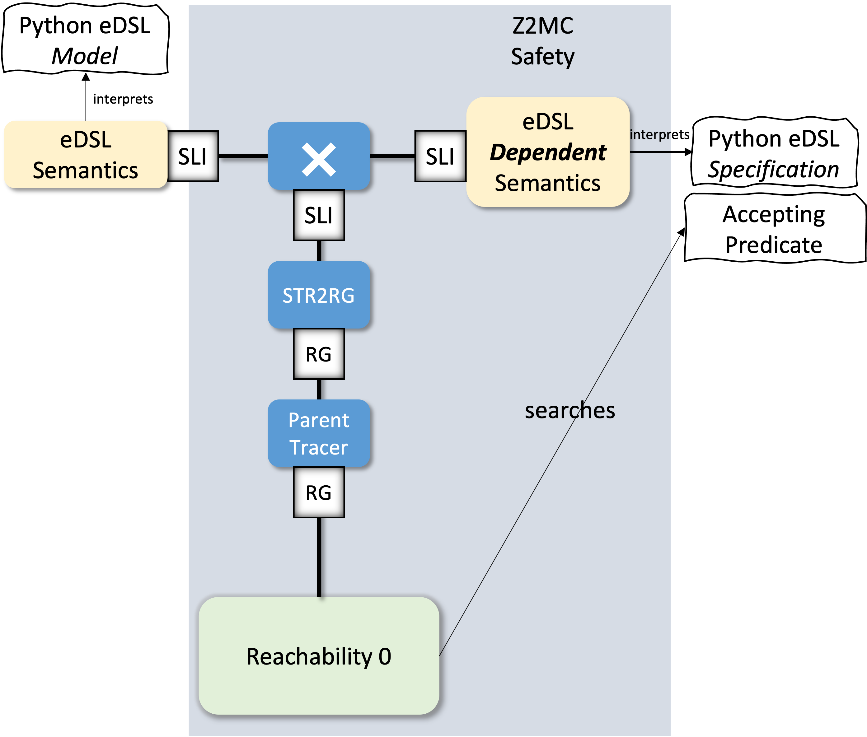
Computing the Intersection Between the System and the Property
 {: width="400" style="display:block; margin-left:auto; margin-right:auto"}
Safety Properties: Looking into the Past
Theoretical approach
- Collect the atomic propositions
- Compute the Kripke structure of the state-space
- Convert the Kripke structure to NFA.
- Compose the system NFA with the property NFA
Let the property compute the Kripke interpretation
- Convert the state-space to a NFA
- Compose the system NFA with the property NFA
Dynamic Composition of the System with the Property
- Dynamically obtain an NFA interpretation of the system during the composition.
class ConfigurationSynchronousProduct(SemanticTransitionRelation):
    def __init__(self, lhs, rhs):
        self.lhs = lhs
        self.rhs = rhs

    def initial(self):
        return list(map(lambda c: (None, c), self.rhs.initial()))

    def actions(self, source):
        synchronous_actions = []
        lhs_source, rhs_source = source
        if source[0] is None:
            for target in self.lhs.initial():
                self.get_synchronous_actions(target, rhs_source, synchronous_actions)
            return synchronous_actions
        # get all lhs actions
        lhs_actions = self.lhs.actions(lhs_source)
        number_of_actions = len(lhs_actions)
        for lhs_a in lhs_actions:
            _, target = self.lhs.execute(lhs_a, lhs_source)
            if target is None:
                number_of_actions -= 1
            self.get_synchronous_actions(target, rhs_source, synchronous_actions)

        # if number_of_actions == 0:
        #     self.get_synchronous_actions(kripke_source, buchi_source, synchronous_actions)
        return synchronous_actions

    def get_synchronous_actions(self, lhs_config, rhs_config, io_synchronous_actions):
        rhs_actions = self.rhs.actions(lhs_config, rhs_config)
        io_synchronous_actions.extend(map(lambda ra: (lhs_config, ra), rhs_actions))

    def execute(self, action, configuration):
        lhs_target, rhs_action = action
        _, rhs_source = configuration
        return kripke_target, self.rhs.execute(rhs_action, lhs_target, rhs_source)
Step Predicates: Looking at execution steps
Expressing conditions on execution steps expands the possibilities for debugging. First of all, the step breakpoints allow us to reason about the action between the configurations. In their simplest form, they can allow stopping the execution when a named action is reached, |action("toOne")|.
Furthermore, the step breakpoints allow reasoning on the delta changes between two consecutive configurations of a behavior (before and after an action). For instance, this will allow us to detect the rising edge of the one-bit clock, |clock=0 && clock'=1|.
class StepSynchronousProduct(SemanticTransitionRelation):
    def __init__(self, lhs, rhs):
        self.lhs = lhs
        self.rhs = rhs

    def initial(self):
        initial_configurations = []
        for lc in self.lhs.initial():
            for rc in self.rhs.initial():
                initial_configurations.append((lc, rc))
        return initial_configurations

    def actions(self, configuration):
        synchronous_actions = []
        # get all lhs actions
        lhs_actions = self.lhs.actions(configuration[0])
        number_of_actions = len(lhs_actions)
        for lhs_a in lhs_actions:
            step, target = self.lhs.execute(lhs_a, configuration[0])
            if target is None:
                number_of_actions -= 1
            rhs_actions = self.rhs.actions(step, configuration[1])
            synchronous_actions.extend(map(
                    lambda ra: (step, ra),
                    rhs_actions
                ))

        if number_of_actions == 0:
            step = (configuration[0], StutteringAction.instance(), configuration[0])
            rhs_actions = self.rhs.actions(step, configuration[1])
            synchronous_actions.extend(map(
                lambda ra: (step, ra),
                rhs_actions
            ))
        return synchronous_actions

    def execute(self, action, configuration):
        step = action[0]
        target = self.rhs.execute(action[1], step, configuration[1])
        return step[2], target
Nested Reachability for Liveness Verification
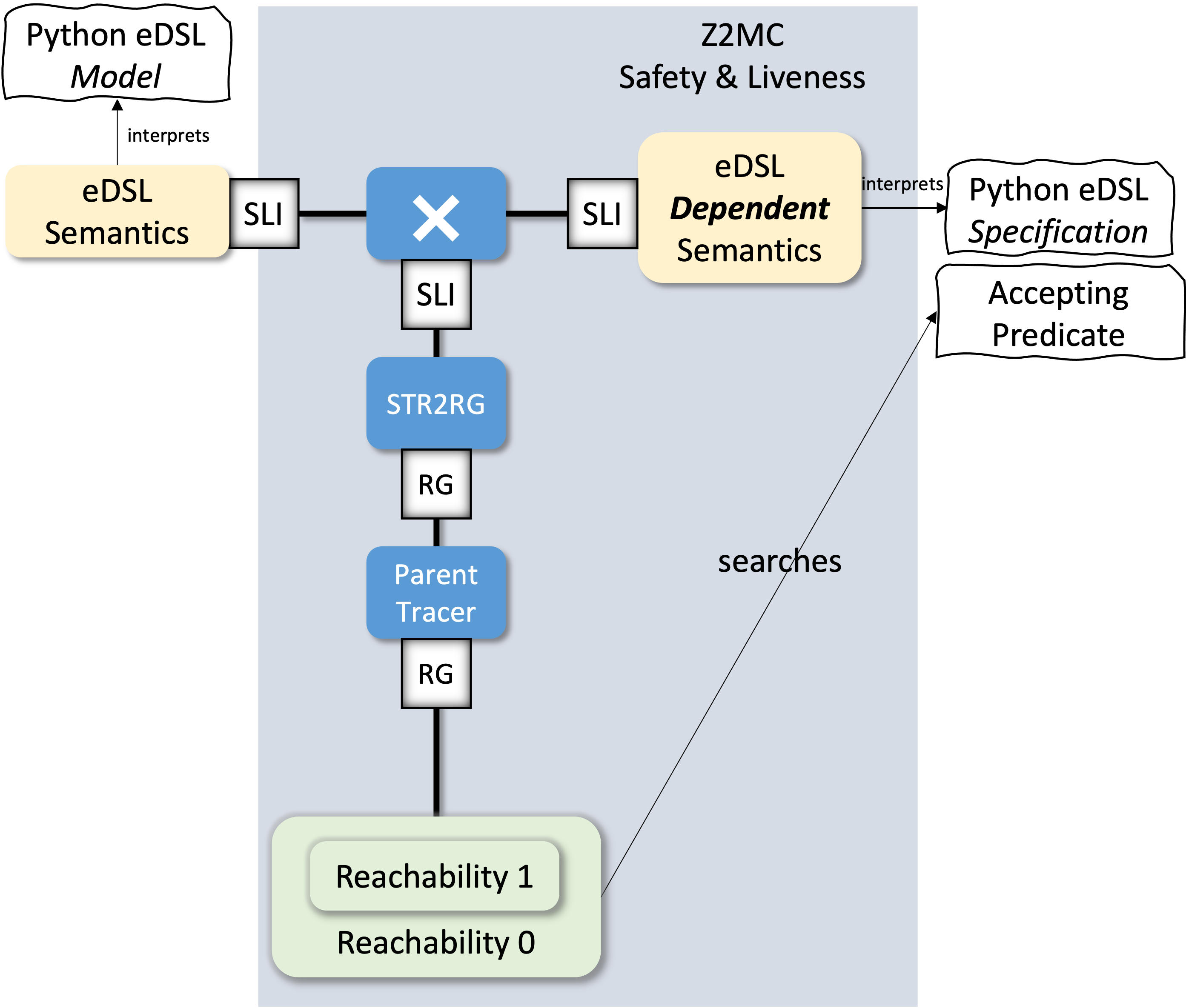 {: width="400" style="display:block; margin-left:auto; margin-right:auto"}
Liveness Properties: Thinking about the Future
Improving Liveness Verification Performance
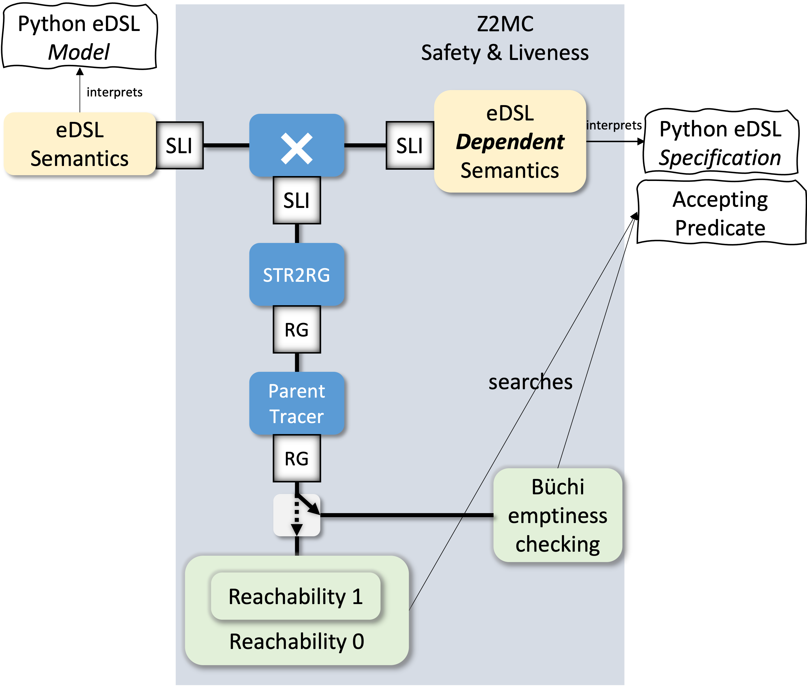 {: width="400" style="display:block; margin-left:auto; margin-right:auto"}
Implement the following state-of-the-art algorithms.

Seeing the Algorithms as Dependent Specifications
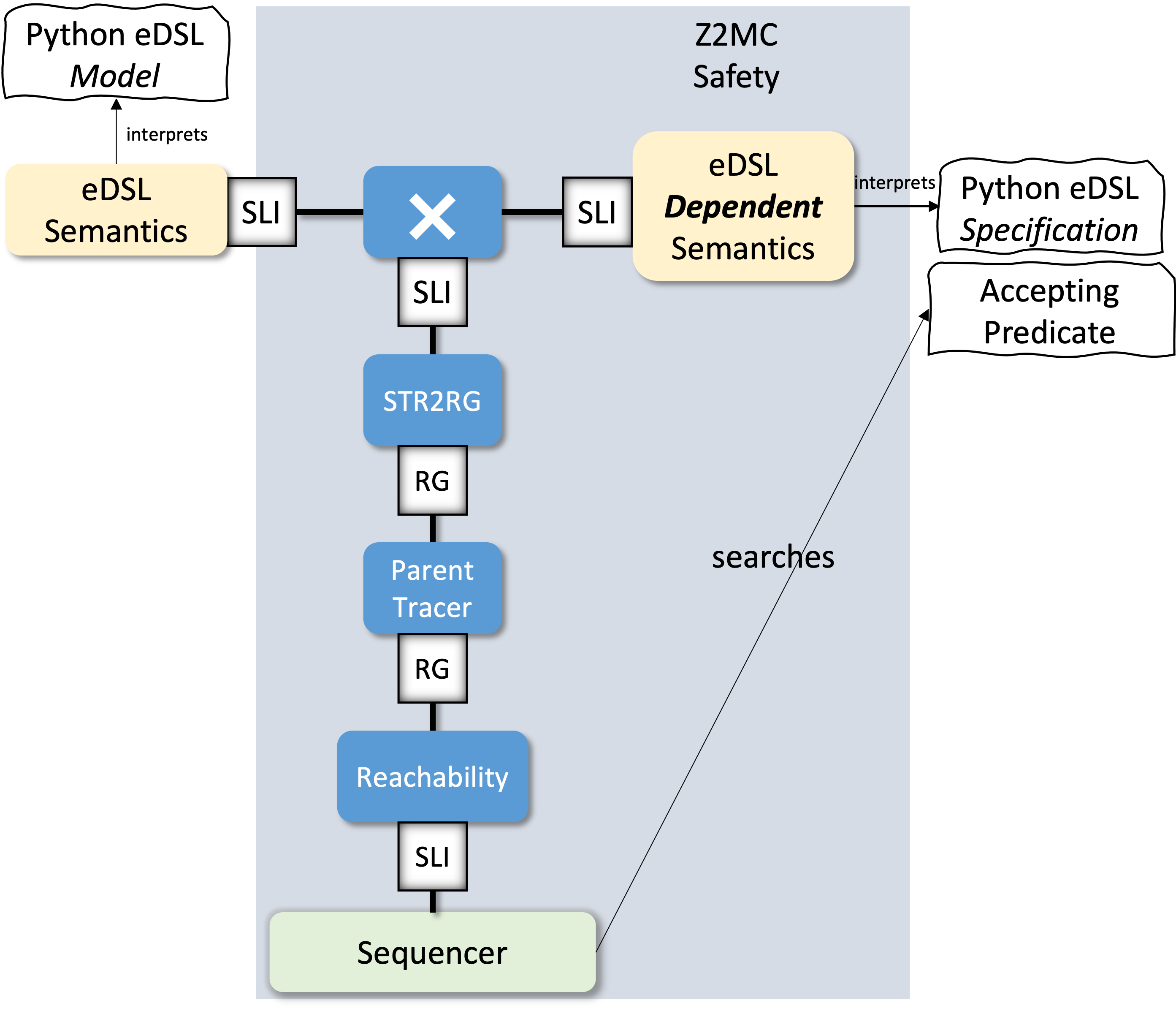 {: width="400" style="display:block; margin-left:auto; margin-right:auto"}